Pivot tables

Total by region, count by status, sales by month, in a minute and without writing a formula.

What a pivot table does

A pivot table takes a clean table (lesson 1) and summarises it: one row per region with the total for each, one row per product with the count of orders, months across the top and categories down the side. It rebuilds itself when the data changes, and it never touches the original rows.

If you are about to write ten SUMIF formulas, one for each region, a pivot table does the same job faster and will not miss the region you forgot.

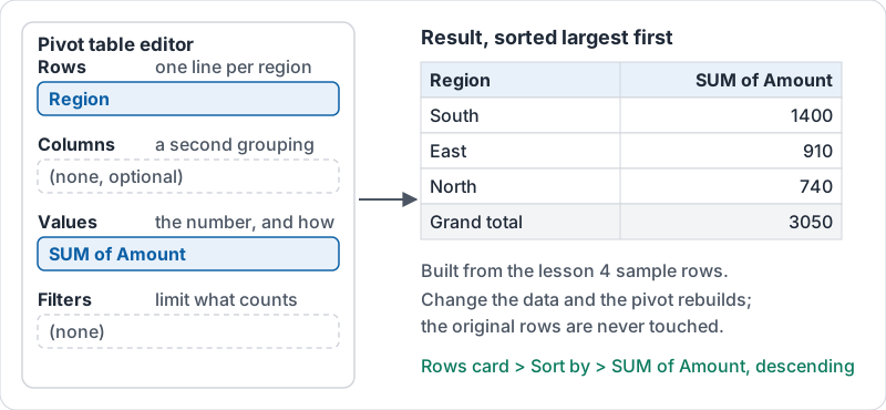
The four boxes

Box	Put here	Example
Rows	The thing you want one line per	Region, Rep, Product
Columns	A second grouping across the top (optional)	Month, Status
Values	The number to summarise, and how	SUM of Amount, COUNT of Order
Filters	Limit what is included	Only Status = Paid

Start simple: one field in Rows, one in Values. Add Columns only when a two-way table genuinely answers the question.

The four boxes and the table they produce from the lesson 4 sample rows.

Rows is what you want one line per; Values is the number and how to summarise it.

SUM, COUNT or AVERAGE

The Values box asks how to summarise. Pick deliberately:

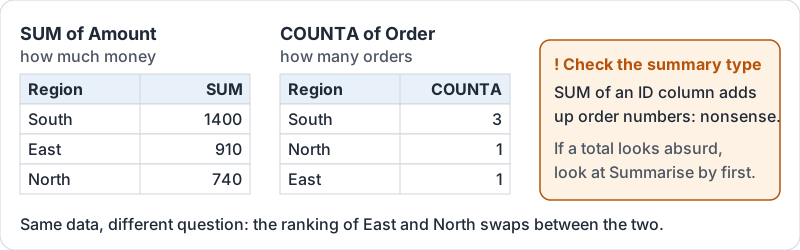
SUM of Amount: how much money per region.
COUNTA of Order (or any text column): how many orders per region.
AVERAGE of Amount: typical order size per region.

A pivot that shows SUM of Order numbers is meaningless; it added up the IDs. If a total looks absurd, check the summary type.

Same data, two summary types, two different rankings.

Two pivot results from the same rows: SUM of Amount gives South 1400, East 910, North 740, while COUNTA of Order gives South 3, North 1, East 1, with a warning box that SUM of an ID column adds up order numbers and means nothing — SUM answers how much; COUNTA answers how many. East and North swap places depending on the question.

Grouping dates by month

A Date column gives one row per day, which is rarely what you want. Group the dates by month or quarter inside the pivot and the rows collapse to “Jan, Feb, Mar”. This only works if the dates are real dates (lesson 1).

Sorting and reading it

Sort the pivot by the Values column, largest first, and the biggest region is on top. The smallest or the biggest drop is then obvious. Put two months in Columns and the comparison sits side by side.

Pivot tables do not update instantly in every case; if the data changed and the pivot looks stale, refresh it or check that the source range still covers all the rows (use whole columns in the source range to avoid this).

How it looks today · Google SheetsChecked Nov 7, 2026

Desktop: click a cell in the data, then Insert > Pivot table and choose New sheet. The pivot editor on the right has Rows, Columns, Values and Filters with Add buttons. In Values, change Summarise by from SUM to COUNTA or AVERAGE as needed. To group dates, right-click a date in the pivot and choose Create pivot date group > Month. Sort from the Rows card using Sort by and Order.

Layout (rolling out from November 2026): the pivot editor is gaining a layout choice. Outline form puts each Rows field in its own column; Compact form nests all the Rows fields in one column with indents and expand/collapse buttons. It changes only how the table looks, not the totals. If you do not see the option yet, it has not reached your account.

Phone (Sheets app): existing pivot tables display and refresh in the app. Create and edit them on a desktop.

Menus and button names change often. If your screen looks different, the skill is the same: look for the equivalent option.

Try it now

On a sales sheet, insert a pivot table on a new sheet with Region in Rows and SUM of Amount in Values. Sort it largest first. Then change the Values summary to COUNTA to see the number of orders per region and notice how different the ranking is.

Remember: Rows is what you want one line per, Values is the number and how to summarise it. Check SUM versus COUNT before you trust a total.

Checking your progress…